Abnormal geological structures, such as fracture zones and faults, are the principal sources of disasters. Precise prediction of unfavorable geological bodies is crucial for tunnel disaster prevention and safety control. The use of a seismic advanced prospecting technique is imperative under adverse conditions. This article looks at Wang, B. & Huang, L.'s study published in Frontiers in Earth Science, which looks at a polarization migration velocity model building method for geological prediction ahead of tunnel faces.
Image Credit: Anna Kucherova/Shutterstock.com
Tunnel Seismic Prediction (TSP) was created by Amberg Company employing three-component receivers in a linear observation system. True Reflection Tomography (TRT) is a technique created by the American NSA Engineering Company. For seismic prediction ahead of a tunnel face, a three-dimensional (3D) observation system is designed.
For assessing the surrounding rock structure and lithological distribution ahead of a tunnel face, velocity data derived from seismic advanced prospecting is essential. As a result, a reflected seismic signal should be utilized to create an accurate velocity model for the unexcavated area before the tunnel face to answer a critical scientific challenge for geological prediction.
There are several challenges faced during the tunneling applications of the advanced prospecting approach. This is due to the difficulties of generating effective lateral offset of the observation system in the confined space of a tunnel, as well as the possibility of faults of various dips and inclinations in the region to be mined, which makes prospecting more difficult.
Using the energy stack method of scattered waves, Amberg Company created an enhanced velocity model with prestack diffraction migration to handle the problem of velocity change in distinct strata ahead of a tunnel face.
To overcome this challenge, this work provides a polarization migration velocity model building (PMVMB) technique. The velocity model ahead of a tunnel face may be developed using this technique by constructing an energy stack on the polarization migration interface while keeping the major polarization angle in mind. The efficiency of this technique was tested using numerical simulations and field trials.
Methodology
The reflected seismic signals obtained by the widely used TSP linear observation system may not collect at a common reflection point (CRP) or common depth point due to the geological dip of a tunnel. Signals originating from nearby reflection points on the same reflection interface will converge at a common interface point (CIP).
Figure 1 shows that the seismic reflected rays create just a single-fold stack; no multifold stack exists.
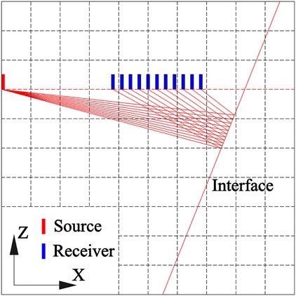
Figure 1. Schematic of seismic wave reflection from slant interface in the advanced detection model. Unlike ground seismic exploration, there are few sources and receivers in tunnel seismic advanced detection. It is difficult to stack in the common reflection point. Image Credit: Wang and Huang, 2022
In this scenario, polarization migration can only generate a reflection energy arc to indicate the position of the reflection interface, not precise reflection spots (Figure 2A). The amplitude of the selected energy arc within the grid is depicted in Figure 2B.
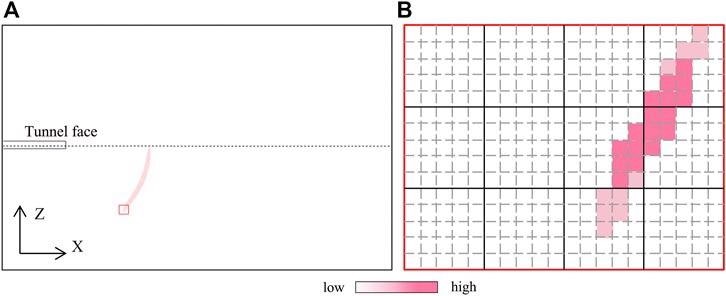
Figure 2. Principle diagram of reflection energy arc of migration. (B) is the partially enlarged schematic diagram of the marked out by the red rectangle in (A). Image Credit: Wang and Huang, 2022
Figure 3 depicts the PMVMB method’s procedure.
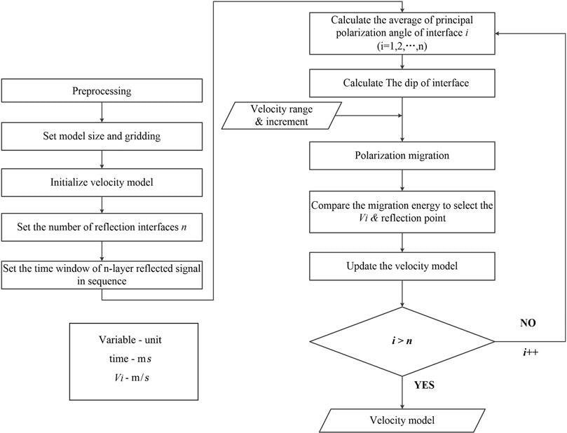
Figure 3. Calculation flowchart of the polarization migration velocity model building method for geological prediction ahead of the tunnel face. Image Credit: Wang and Huang, 2022
The red square in Figure 4B represents the source position; the blue squares represent the 16 receivers designated R1-R16; and the last receiver is on the tunnel face. The slightly expanded schematic of the tunnel and observation system illustrated in Figure 4B is shown in Figure 4C.
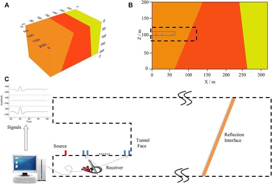
Figure 4. Geological model and seismic observation system. (A) 3D geological model; (B) XOZ diagrammatic cross-section; (C) The partially enlarged schematic diagram of observation system. Image Credit: Wang and Huang, 2022
The system is numerically simulated using the finite difference approach; the model is displayed in Figure 5 and the parameters are listed in Table 1.
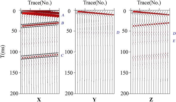
Figure 5. Simulated three-component seismic records of advanced detetion. Image Credit: Wang and Huang, 2022
Table 1. Model parameters. Source: Wang and Huang, 2022
| No. |
Velocity of P-wave (m/s) |
Interface |
Distance (m) |
Degree (°) |
| I |
3,800 |
F1 |
101 |
-69 |
| II |
4,100 |
F2 |
253 |
83 |
| III |
4,500 |
- |
- |
- |
The particle polarization trajectory derived from the P-wave signal reflected from the first interface and captured by the second three-component receiver is depicted in Figure 6A. Many energy arcs are almost parallel to each other on one side of the axis in Figure 6B. The energy-velocity curve may be generated by superposing the energy arcs for different velocities (Figure 6C). The R1 interface (Figure 6D) is 98 m long, has a negative slope, and has a 65° dip.
![Polarization migration results of the first interface. (A) represents the particle vibration of No. 2 receiver, whose principal polarization angle is -25°. The polarization migration results in (B) are obtained by superposing all the 16 receivers. Since the migration results corresponding to 15 velocities [in part (C)] are difficult to display, the polarization migration interfaces corresponding to five velocities at relatively large intervals are selected. According to the velocity of Vp in (C) and the principle polarization angle in (A), polarization migration interface is confirmed.](https://www.azomining.com/images/Article_Images/ImageForArticle_1642_16469093045225710.jpg)
Figure 6. Polarization migration results of the first interface. (A) represents the particle vibration of No. 2 receiver, whose principal polarization angle is −25°. The polarization migration results in (B) are obtained by superposing all the 16 receivers. Since the migration results corresponding to 15 velocities [in part (C)] are difficult to display, the polarization migration interfaces corresponding to five velocities at relatively large intervals are selected. According to the velocity of Vp in (C) and the principle polarization angle in (A), polarization migration interface is confirmed. Image Credit: Wang and Huang, 2022
Figure 7A shows the results of the migration study with a period length of 110.4–117.07 ms. Figure 7B depicts the migration outcomes at various speeds while the primary polarization angle is held constant. Figure 7C shows the results of processing the polarization migration data of the five velocities using energy superposition and the energy-velocity curve. Figure 7D shows the R2 interface, which is positioned at 257 m, is favorably sloped, and has a 78° dip.
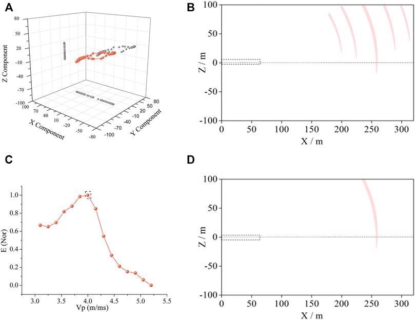
Figure 7. Polarization migration results of the second interface. (A) represents the particle vibration of No. 2 receiver. The polarization migration results in (B) are obtained by superposing all the 16 receivers. Since the migration results corresponding to 15 velocities (in part (C)) are difficult to display, the polarization migration interfaces corresponding to five velocities at relatively large intervals are selected. According to the velocity of Vp in (C) and the principle polarization angle in (A), polarization migration interface is confirmed. Image Credit: Wang and Huang, 2022
The correct polarization migration results of the two interfaces are shown in Figure 8.
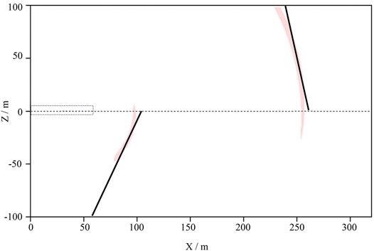
Figure 8. Polarization migration results of two reflection interfaces. The polarization migration results of the two-layer interface can be obtained, as shown in the red arc in the figure. Under the control of the principal polarization angle, the interface angles of the two layers are 65° and 78° respectively. The black lines are tangent to the red arcs and in line with the angle, and the lines are selected to the location of the reflection interfaces. Image Credit: Wang and Huang, 2022
Based on the reflection interfaces and velocities, a velocity model is built and displayed in Figure 9.
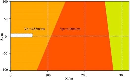
Figure 9. Velocity model of PMVMB method. The rightmost area represents the third layer of the model whose left boundary is defined by Figure 7D. Since there is no reflection interface on the rightmost area of the model, no reflected signals can be received. Accordingly, background velocity can be used as the velocity in this area because there is no way to solve the velocity of this area. Image Credit: Wang and Huang, 2022
Figure 10A depicts the precise position. The Maanshan tunnel, the project’s longest tunnel, runs from K0 +273.0 to K12 + 473.0.
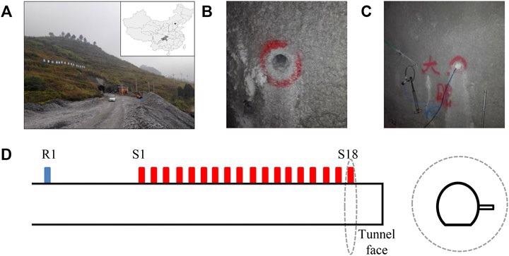
Figure 10. Layout of seismic observation system in Maanshan tunnel. (A) is the tunnel location. (B) is the layout of the blasthole. (C) is the position of the geophone. (D) is the schematic diagram of the observation system, and inside the dotted line is a cross section of the tunnel. Image Credit: Wang and Huang, 2022
Figure 11A shows R1’s common receiver gathers of the X component.
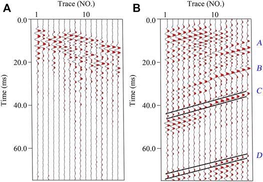
Figure 11. Original and preprocessed seismic record. Two events marked by black lines in (B) are selected as calculation signals of PMVMB method. Image Credit: Wang and Huang, 2022
Figure 12 shows how early prospecting data and direct wave velocity may be used to create a velocity model for the excavated region.
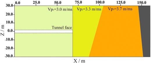
Figure 12. Velocity model and polarization migration results of PMVMB method. Since there are only two layers of reflected signals in Figure 11, the seismic wave velocity in the rightmost area in this figure cannot be determined. Image Credit: Wang and Huang, 2022
Discussion
Three-component seismic wave receivers were arranged to pick up reflected seismic waves using the commonly utilized TSP linear observation technique. With three-component reflected signals, the PMVMB approach can reliably determine the velocity and location of reflection interfaces.
The PMVMB approach is based on CIP’s energy stack characteristics, which allows the velocity model to be correctly established.
The PMVMB approach has an advantage over other methods in that it makes use of the vector properties of three-component seismic signals. The technique calculates the primary energy direction of reflected wave propagation by using matrix analysis to derive the principal polarization direction.
In this work, researchers just looked at how to develop a P-wave velocity model. The procedure for creating S-wave velocity models is the same, and the assumption is the separation of P-wave and S-wave.
Conclusion
This paper explains the PMVMB technique in theory and provides the calculation principle for removing the symmetric interface artifact via Hilbert polarization migration. Researchers also presented a method for identifying the best velocity based on CIP gather’s energy stack characteristics.
The experimental findings show that the PMVMB technique can handle real-world issues, including erroneous velocity calculations in the stratum ahead of the tunnel face and migration artifacts. These results have practical implications for the identification of high-dip faults.
Journal Reference:
Wang, B. & Huang, L. (2022) A Polarization Migration Velocity Model Building Method for Geological Prediction Ahead of the Tunnel Face. Frontiers in Earth Science, p.299. Available Online: https://www.frontiersin.org/articles/10.3389/feart.2022.857984/full.
References and Further Reading
- Ashida, Y &Sassa, K (1993) Depth Transform of Seismic Data by Use of Equi-Travel Time Planes. Exploration Geophys,24, pp. 341–346. doi.org/10.1071/EG993341.
- Bellino, A., et al. (2013) An Automatic Method for Data Processing of Seismic Data in Tunneling. Journal of Applied Geophysics, 98, pp. 243–253. doi.org/10.1016/j.jappgeo.2013.09.007.
- Brossier, R (2011) Two-dimensional Frequency-Domain Visco-Elastic Full Waveform Inversion: Parallel Algorithms, Optimization and Performance. Computer Sciences and Geosciences,37(4), pp. 444–455. doi.org/10.1016/j.cageo.2010.09.013.
- Buske, S., et al. (2009) Fresnel Volume Migration of Single-Component Seismic Data. Geophysics, 74(6), pp. WCA47–WCA55. doi.org/10.1190/1.3223187.
- Chao, L., et al. (2021) A Comprehensive Evaluation of Five Evapotranspiration Datasets Based on Ground and grace Satellite Observations: Implications for Improvement of Evapotranspiration Retrieval Algorithm. Remote Sensing,13(12), p. 2414. doi.org/10.3390/rs13122414.
- Cheng, F., et al. (2014) Two-dimensional Pre-stack Reverse Time Imaging Based on Tunnel Space. Journal of Applied Geophysics, 104, pp. 106–113. doi.org/10.1016/j.jappgeo.2014.02.013.
- Diallo, M. S., et al. (2006) Instantaneous Polarization Attributes Based on Adaptive Covariance Method. Geophysics, 71, p. V99. doi.org/10.1190/1.2227522.
- Dickmann, T & Sander, B K (1996) Drivage-concurrent Tunnel Seismic Prediction (TSP). Felsbau 14 Nr, 6, pp. 406–411.
- Esmailzadeh, A., et al. (2018) Prediction of Rock Mass Rating Using TSP Method and Statistical Analysis in SemnanRooziyeh spring Conveyance Tunnel. Tunnelling and Underground Space Technology, 79, pp. 224–230. doi.org/10.1016/j.tust.2018.05.001.
- Fan, Y., et al. (2021) Rockburst Prediction from the Perspective of Energy Release: A Case Study of a Diversion Tunnel at Jinping II Hydropower Station. Frontiers in Earth Science, 9, p. 711706. doi.org/10.3389/feart.2021.711706.
- Gong, X.-B., et al. (2010) Combined Migration Velocity Model-Building and its Application in Tunnel Seismic Prediction. Applied Geophysics, 7, pp. 265–271. doi.org/10.1007/s11770-010-0251-3.
- Grechka, V., et al. (2002) Multicomponent Stacking‐velocity Tomography for Transversely Isotropic media. Geophysics, 67, pp. 1564–1574. doi.org/10.1190/1.1512802.
- Huang, X., et al. (2021) Multi-step Combined Control Technology for Karst and Fissure Water Inrush Disaster during Shield Tunneling in spring Areas. Frontiers in Earth Science, 9, p. 795457. doi.org/10.3389/feart.2021.795457.
- Inazaki, T., et al. (1999) Stepwise Application of Horizontal Seismic Profiling for Tunnel Prediction Ahead of the Face. The Leading Edge, 18, pp. 1429–1431. doi.org/10.1190/1.1438246.
- Joudaki, V., et al. (2018) Evaluation of Tunnel Seismic Prediction (TSP) Test Results Based on Geological Observations and Analysis of the Parameters of the EPB Hard Rock Machine. Journal of Iranian Association of Engineering Geology,11, pp. 15–31.
- Kneib, G., et al. (2000) Automatic Seismic Prediction Ahead of the Tunnel boring Machine. First Break, 18(7), pp. 295–302. doi.org/10.1046/j.1365-2397.2000.00079.x.
- Koren, Z & Ravve, I (2006) Constrained Dix Inversion. Geophysics, 71, pp. R113–R130. doi.org/10.1190/1.2348763.
- Lambrecht, L & Friederich, W (2013) “Forward and Inverse Modeling of Seismic Waves for Reconnaissance in Mechanized Tunneling,” in EGU General Assembly Conference Abstracts, 15, p. 4376L.
- Li, S. C., et al. (2015) Comprehensive Geophysical Prediction and Treatment Measures of Karst Caves in Deep Buried Tunnel. Journal of Applied Geophysics, 116, pp. 247–257. doi.org/10.1016/j.jappgeo.2015.03.019.
- Li, S., et al. (2017) An Overview of Ahead Geological Prospecting in Tunneling. Tunnelling and Underground Space Technology, 63, pp. 69–94. doi.org/10.1016/j.tust.2016.12.011.
- Liu, B., et al. (2017) Three-dimensional Seismic Ahead-Prospecting Method and Application in TBM Tunneling. Journal of Geotechnical & Geoenvironmental Engineering,143(12), p. 04017090. doi.org/10.1061/(ASCE)GT.1943-5606.0001785.
- Liu, B., et al. (2020) Mapping Water-Abundant Zones Using Transient Electromagnetic and Seismic Methods when Tunneling through Fractured Granite in the Qinling Mountains, China. Geophysics, 85(4), pp. 147–159. doi.org/10.1190/geo2019-0067.1.
- Liu, Y & Mei, R (2011) Advantages of TGP advance Geology Prediction Technology in Tunnels. Tunnel construction machinery (Chinese Edition), 31(1), pp. 21–32.
- Lüth, S., et al. (2008). “A Seismic Exploration System Around and Ahead of Tunnel Excavation–Onsite,” in World Tunnel Congress, Agra, India, pp. 119–125.
- Otto, R., et al. (2002) The Application of TRT-True Reflection Tomography-At the Unterwald Tunnel. Felsbau, 20, pp. 51–56.
- Prabhakaran, A & Jawahar Raj, N (2018) Mapping and Analysis of Tectonic Lineaments of Pachamalai hills, Tamil Nadu, India Using Geospatial Technology. Geology, Ecology, and Landscapes, 2(2), pp. 81–103. doi.org/10.1080/24749508.2018.1452481.
- Tzavaras, J., et al. (2012). Three-dimensional Seismic Imaging of Tunnels. International Journal of Rock Mechanics and Mining Sciences, 49, pp. 12–20. doi.org/10.1016/j.ijrmms.2011.11.010.
- Wang, B., et al. (2020) A Hilbert Polarization Imaging Method with Breakpoint Diffracted Wave in Front of Roadway, Journal of Applied Geophysics, 177, pp. 1–9. doi.org/10.1016/j.jappgeo.2020.104032.
- Wang, B., et al. (2021) Seismic Wave Field Characteristics and Application of CO2 Concentrated Force Source. Journal of China Coal Society, 46(2), pp. 556–565. doi.org/10.1016/j.ijggc.2014.12.009.
- Wang, E., et al. (2016) Reverse Time Migration Using Analytical Wavefield and Wavefield Decomposition Imaging Condition. ActaGeodynamica, 13, pp. 1–12. doi.org/10.1190/segam2016-13823057.1.
- Wang, Y., et al. (2019) Application of a New Geophone and Geometry in Tunnel Seismic Detection. Sensors, 19, p. 1246. doi.org/10.3390/s19051246.
- Xiao, Q H & Xie, C J (2012) Application of Tunnel Seismic Tomography to Tunnel Prediction in Karst Area. Rock and Soil Mechanics, 33(5), pp. 1416–1420.
- Yamamoto, T., et al. (2011) Imaging Geological Conditions Ahead of a Tunnel Face Using Three-Dimensional Seismic Reflector Tracing System. International Journal of Research in Commerce and Management, 6, pp. 23–31. doi.org/10.11187/ijjcrm.6.23.
- Zeng, Z H (1994) Prediction Ahead of the Tunnel Face by the Seismic Reflection Methods. Chinese Journal of Geophysics –CH, 37, pp. 218–230.
- Zhang, K., et al. (2019) Characteristics and Influencing Factors of Rainfall-Induced Landslide and Debris Flow Hazards in Shaanxi Province, China Natural Hazards and Earth System Sciences,19(1), pp. 93–105. doi.org/10.5194/nhess-19-93-2019.
- Zhao, Y. G., et al. (2008) The Technical Bug of TSP203 and Application of TST Technique. Chinese Journal of Engineering Geophys, 3, pp. 15–22.
- Zhao, Y., et al. (2006) Tunnel Seismic Tomography Method for Geological Prediction and its Application. Applied Geophysics, 3, pp. 69–74. https://doi.org/10.1007/s11770-006-0010-7.
- Zhou, G., et al. (2021) Selection of Optimal Building Facade Texture Images from UAV-Based Multiple Oblique Image Flows. IEEE Trans. Geoscience and Remote Sensing, 59(2), pp. 1534–1552. doi.org/10.1109/TGRS.2020.3023135.