This article explores the use of three new automated mineralogy features. These features can provide ZIESS Mineralogic Mining with several distinct capabilities that are especially useful when tackling many of the mineral processing challenges present in modern-day mining operations. These are:
Quantitative Measurement of the Chemical Composition of Minerals
This function can automatically detect the presence of specific elements in any X-ray spectrum for a measured mineral. It is then able to calculate the amount of each element and its quantitative abundance. This extremely useful quantitative data can then be used as the basis for calculated sample assay and mineral classification.
Combined Morphological and Chemical Classification
SEM techniques are typically used to classify minerals on the basis of chemistry, but this additional functionality allows for further subdivision of isochemical minerals based on morphology (textural characteristics).
This analysis is taken from a high-quality BSE image and can distinguish, for example, massive low-porosity muscovite vs fine-grained porous sericite or course ‘vein’-related chalcopyrite vs fine disseminated chalcopyrite.
Lithology Classification
Mineralogy data can be placed back into a lithological context via particle classification functionality. This functionality is based on:
- Constituent mineralogy
- Area of the constituent mineralogy
- Particle area
- Particle exposed perimeter per mineral
- Particle porosity
As well as being useful lithological classifications, these classifications can report on the assay per lithology by using either normalized, standardless EDX or standards-based EDX made from chemical mineral and combined morphological classifications.
Unique Features Explained
Quantitative Measurement of the Chemical Composition of Minerals
The Mineralogic platform uses quantitative chemical composition as its foundation, using a fast, single pass X-ray analysis to ensure that the composition of every pixel is analyzed appropriately. The measured composition is then assigned to each individual pixel and classified according to the system’s library of minerals.
This technique is different from other approaches such as automated mineralogical classification which may use the unquantified presence of a particular chemical element to classify analyses.
The Mineralogic approach to classification offers a range of distinct advantages including the following:
Firstly, solid-solution variations commonly found in a range of mineral groups like amphiboles, micas, chlorites, and pyroxenes are measured directly; meaning these do not need to be approximated or inferred.
Secondly, because every pixel analyzed is then quantified, the chemical composition can be analyzed to a high degree of accuracy. This is different and preferable to existing methods, where expected compositions of minerals must be pre-assigned and only a single composition per mineral entry can be used for the whole sample.
When this functionality is used alongside lithology classifications, real and tangible chemical differences between lithologies can be ascertained and measured; for example, a coarse-grained muscovite-dominant lithology within a porphyry-copper deposit could contain higher amounts of fluorine than a fine-grained ‘secondary’ sericite-dominant lithology.
This method of quantified chemical analysis ensures that much simpler mineral libraries can be created. In situations where a variety of solid solution chemical variants are expected to be present, other techniques would require separate entries for each composition to capture the full range of compositions present.
In cases where the association and liberation of the different end-members of the solid solution is not important or does not need to be known, Mineralogic classifications only need a single entry for the specific solid solution.
Of particular benefit is the fact that when using the Mineralogic approach, there is no need to have full prior knowledge of all the elements that might be present in a particular sample. There is no need to know this beforehand because any elements present (such as Zn in pyrite) will be captured and reported if they are detected.
In order to ensure maximum accuracy with mineral classification schemes, these may require some iterative improvements as unexpected elements are discovered, but all chemical-element data are retained, and samples can therefore be retrospectively reprocessed as the mineral library is optimized and improved.
Mineralogic offers two spectrum quantification methods: normalized standard-less quantification and standards-based quantification.
Standardless quantification can accommodate a quick and simple workflow that is especially suitable for heavier elements, but it does lack the chemical accuracy that is afforded by using standards-based calibrations.
Mineralogic can offer comprehensive standards-based quantification without normalization. This utilizes the same approach as standards-based electron microprobe techniques (including the μoe, øρZ or ZAF matrix correction); providing consistent, accurate data with the overall results suffering no adverse impact due to the presence of unmeasurable elements.
There is however a need for a certified homogeneous standard to be present for each element, and element lines present in each standard must be free of background artifacts or significant interference for this approach to be used successfully.
Methodology
During these examples, the standards-based calibration used has been based on the certified reference standard 7609, provided by MAC (Micro-Analysis Consultants Ltd, UK).
Table 1. Element standards used for standards-based quantification using Bruker Esprit integrated with Mineralogic; all but the phosphorous standards are available on the MAC Registered Standard No. 7609
| Element |
MAC 7609 Standard |
| Si |
Wollastonite |
| Al |
Corundum |
| Ti |
Ti metal |
| Fe |
Pyrite |
| Mn |
Mn metal |
| Mg |
Periclase |
| Ca |
Wollastonite |
| Na |
Jadaite |
| K |
Orthoclase |
| P |
AlPO4 compound* |
| S |
Pyrite |
| Cu |
Cu metal |
| As |
InAs compound |
| Zn |
Zn metal |
* Rio Tinto standard, not provided by MAC
Here, an iron ore sample (~48 frames, 0.25 second dwell time) containing hematite and goethite has been measured using both the standards-based quantification and default normalized quantification methods.
These results are compared to a reference value in the figures below. It is worth noting here that the top and bottom of each box represents that 1st and 3rd quartiles respectively, while the bar is the median value. The whiskers shown reach out to the minimum and maximum values of the data up to 1.5 box lengths with any extra data points being plotted separately as outliers.
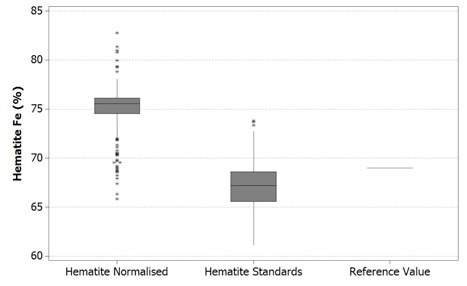
Figure 1. Boxplot of Fe values in hematite using Mineralogic normalized quantification (left) and standards-based quantification (middle) and comparison with the stoichiometric iron value for hematite (right)
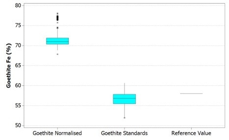
Figure 2. Boxplot of Fe values in goethite using Mineralogic normalized quantification (left) and standards-based quantification (middle) and comparison with a reference value of typical Pilbara goethite (right)
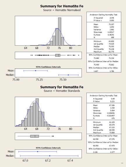
Figure 3. Statistical comparison of hematite results obtained from normalized (top) and standards-based (bottom) quantification.
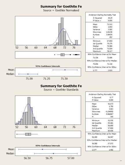
Figure 4. Statistical comparison of goethite results obtained from normalized (top) and standards-based (bottom) quantification
These reference values are, however not the same grains used in the Mineralogic automated measurements. The hematite reference value is in fact the stoichiometric iron value for this mineral while the goethite reference value is actually the average of a small number of in situ quantitative analyses on a typical Pilbara goethite (collected separately, without using Mineralogic).
Normalized, standardless quantified results produce higher iron values for both these iron oxide minerals because there are only two major X-ray peaks present in the spectrum; those peaks being iron and oxygen. The oxygen peak is especially sensitive to surface features, absorption, and detector solid angle through the detector window, so this is always low and variable.
The normalization calculation artificially increases the result for the iron in relation to oxygen while the hydrogen in the goethite is not taken into account, further adding to this systematic error.
The same results are shown statistically in the following figures. Here, it can be observed that in both cases the normalized data show higher variability – that is, there is a clear mismatch between the mean and the median values for the normalized results. This occurs due to the variability in the height of the oxygen peak between one analysis and the next.
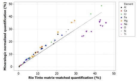
Figure 5. Correlation of Mineralogic normalized quantification values with Rio Tinto reference values for indicator minerals; note that oxygen is systematically low which results in the other elements being systematically high using this method
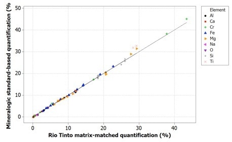
Figure 6. Correlation of Mineralogic standards-based quantification values with Rio Tinto reference values for indicator minerals; oxygen is not measured (and therefore not shown) but is calculated from stoichiometry.
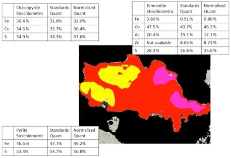
Figure 7. Mineralogic classified images of a composite sulfide particle comparing the standards-based and normalized quantification results with the expected stoichiometric values for three sulfide minerals; note that the tennantite grain contains significant zinc and is not directly comparable with the stoichiometric value.
An additional, secondary comparison was completed using a Rio Tinto secondary standard for diamond indicator minerals. This particular standard is used for regular quality control within exploration applications, with quantitative data for each mineral being verified via two different analytical techniques using specific matrix-matched standards.
Reference values are shown here on the X-axis, then compared via a one-to-one correlation line with both results from normalized quantification and the results gained from standards-based quantification.
It should be noted that all the quantitative data from Mineralogic has been taken from a fast, single pass X-ray analysis with a dwell time of around 0.05 seconds. This would, of course, have much lower levels of accuracy than a more precise, 2-minute electron microprobe analysis.
Oxygen values are generally too low when using normalized quantification, causing all the remaining elements to be measured too highly; while on the other hand, the data for the standards-based quantification tends to be in agreement with the reference values.
It should also be noted that for the latter data, oxygen has not been measured from the X-ray peak because of the previously stated issues with low accuracy and precision. These data use oxygen calculations from stoichiometry.
A complicated statistical analysis of major and trace element data indicator minerals is used to decide upon positive vs negative exploration targets. Major element data is used for internal-standard correction of the trace element data, which is taken directly from the LA-ICPMS system.
In this case, normalized Mineralogic results would not be accurate enough to be utilized in routine exploration applications. However, the standards-based quantification available in the current version of Mineralogic more than meets these accuracy requirements.
The last comparison shown has been completed interactively on sulfide minerals found within a copper deposit. The values displayed are shown on the classified Mineralogic image of a composite sulfide particle while the normalized vs. standards-based vs. stoichiometric values are contrasted for each mineral shown.
As can be seen, the normalized results face similar challenges to accuracy, though in this case the errors are not as prominent because of a lack of light elements which are generally harder to measure.
Combined Morphological and Chemical Classification
‘Morphochemical’ classification is an especially useful and new functionality that enables users to subdivide isochemical minerals even further. It allows these to be sorted based on morphological measurements – that is, textural characteristics, obtained in a similar way to a high-quality BSE image.
The software needs a ‘base’ mineral definition. This is constructed from common chemical classification criteria which is then extended in scope to also capture textural differences.
To give a basic example of this functionality, one can look at grain size. Chalcopyrite can be split into fine and coarse grains, with the mineralogical and petrological characteristics of each of these types queried and examined separately, such as looking at their association with gangue, liberation etc.
A variety of other common textural characteristics can be quantitively measured and used for classification - these include surface area, roughness, grain shape and porosity.
To give a practical example of this morphochemical classification, a classification can be generated in Mineralogic for a target mineral such as ‘roanokite’. The first step of this process is the entering of a chemical composition for the mineral. Next, various subdivisions can be added, such as using the morphological parameter of ‘compactness’ to then distinguish between ‘clean roanokite’, ‘rough roanokite’ and ‘dirty roanokite’. See the following figures for a more graphical illustration of this process.
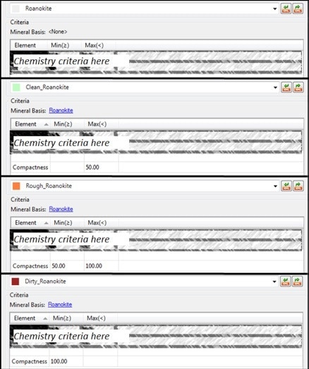
Figure 8. Mineralogic morphochemical classification of “roanokite” on the basis of compactness; the top classification is based on chemistry alone and forms the “base” mineral for the other three entries which are divided into “compactness” intervals.
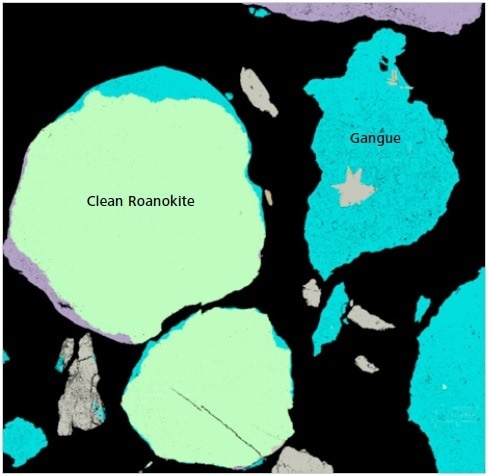
Figure 9. Classified Mineralogic image to show the nature of “clean roanokite”.
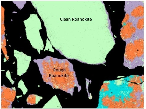
Figure 10. Classified Mineralogic image to show the differences between “clean roanokite” and “rough roanokite”; the latter is less liberated and contains very fine gangue inclusions that will be released into the slurry as the target mineral is digested through leaching.
The key visual difference between these different morphological types is the presence of a large number of tiny gangue inclusions in both the ‘rough’ and ‘dirty roanokite’.
This difference results in a range of quantitative compactness values being measured by Mineralogic. Here, compactness is a measurement of how close each pixel within a grain is in relation to every other pixel. In this example, rounded blogs have a low compactness value while more complex or convoluted shapes can be considered to have higher compactness values.
This particular ore is beneficiated via leaching and comminution, and these distinct differences in its morphology can impact processing behavior. Major downstream tailings density can be impacted by the release of the especially fine gangue into the slurry as the ‘rough roanokite’ is digested during processing.
The following table examines the quantitative results for two samples of the aforementioned ore. Here, the morphochemical classification of these very different types of ‘roanokite’ has enabled them to be separately distinguished; meaning that these two ore types can be handled appropriately and in line with their very distinct properties.
Table 2. Mineralogic results for two samples that contain distinctly different abundances of different morphological types of the same mineral
| Mineral |
Sample 1 (wt%) |
Sample 2 (wt%) |
| Clean Roanokite |
31.2 |
46.7 |
| Rough Roanokite |
1.8 |
28.7 |
| Carbonate |
55.8 |
1 |
| Sulphide |
0.2 |
0.3 |
| Gangue |
11.1 |
23.2 |
| Total |
100 |
100 |
If the mineral had been classified solely on the basis of its chemical composition, this advanced classification would not be possible.
Please note that ‘roanokite’ is not a real mineral name, and specific chemical classification criteria are not shown here for reasons of commercial sensitivity.
Lithology Classification
Within Mineralogic, lithology is dictated by particle classification based on the proportions of the constituent minerals ± particle surface area (partial perimeter) ± particle porosity for each particle.
Examples showing different lithologies from a copper deposit are shown below. These examine the deposit based on porosity and mineralogy. Additionally, bulk modal mineralogy and total calculated chemical assay are standard measurements used within every mineralogical analysis technique.
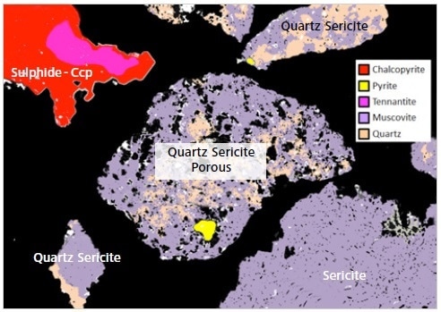
Figure 11. Mineralogic classified image with labels of various “lithologies” from a copper deposit in a single frame; note that the “quartz sericite” lithology in this example can be separated by a quantitative measure of the overall particle porosity.
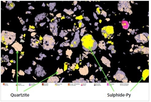
Figure 12. A screenshot of an image “montage” created in Mineralogic Explorer to show sulfide and quartzite lithologies from a copper deposit
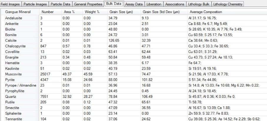
Figure 13. Screenshot of the bulk modal mineralogy table in Mineralogic Explorer, including the average chemical composition for each mineral as directly measured using standards-based quantification.
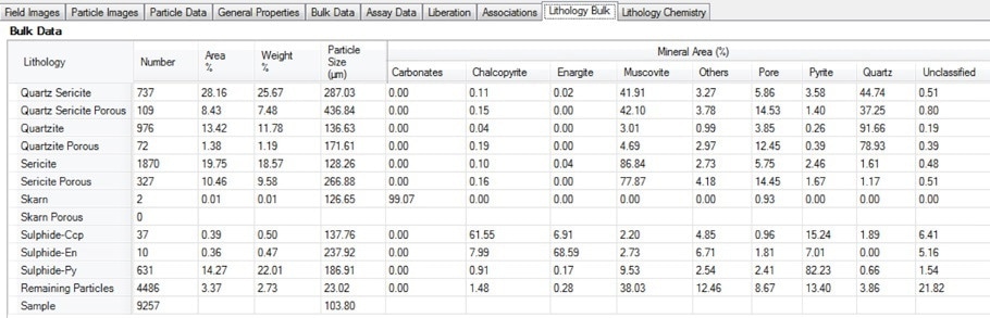
Figure 14. Screenshot of the bulk lithology table in Mineralogic Explorer; the average mineralogy by area % for each user-defined lithology is calculated separately, including a quantitative measure of particle porosity.
Mineralogic can export the average mineralogy, including porosity, for every separate lithology in a sample. It can also export the average chemical assay for each of these lithologies.
In the example below, note how chalcopyrite levels in porous quartzite are highest, but much lower than in the (low-porosity) quartzite.
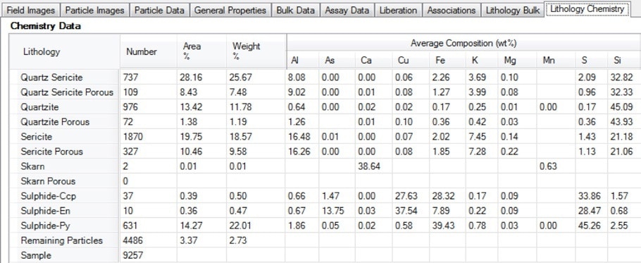
Figure 15. Screenshot of the lithology chemistry table in Mineralogic Explorer; deportment of valuable or deleterious elements can be separated by lithology using this functionality
This export functionality has the scope to add considerable value to any ore characterization project that uses coarse fractions. It is especially useful where important geometallurgical properties (such as particle porosity, percentage of acid consuming minerals, percentage of hard minerals etc.) are measured using the SEM before being linked back to lithological domains in the block model and the ore body.
Lithology classification cannot be applied to fine fractions. This is because, below a certain size, crushed parties are separated into the constituent minerals and any lithological context is then lost.
Conclusion and Recommendations
The normalized quantification method is used in many operations where its ease of use, speed benefits and acceptable results with heavier elements are of a particular advantage. However, incorporating standards-based quantification in Mineralogic can add immense value to this process including much higher accuracy during the analysis of iron minerals and light elements.
Additionally, morphochemical classification is a valuable feature when used to identify textural differences in ore samples. Its range of applications is set to be expanded greatly in the future, meaning that morphological parameters will be able to be set as ratios of two image analysis measurements rather than just as fixed ranges of individual analysis measurements.
Lithology classifications are especially utilized in ore characterization projects that use coarse fractions, and the option to then report the standards-based quantification of assay per lithology offers tremendous potential for value generation across a wide range of commodities.
To summarize, the Mineralogic system is able to provide a selection of distinct and unique features that offer considerable scope for value generation across the whole mining value chain.
The software has been in continuous development since its launch in 2014 and the technology is looking to have a very promising future; already offering significant advantages over similar methods, as has been highlighted and validated within the study outlined above.

This information has been sourced, reviewed and adapted from materials provided by Carl Zeiss Microscopy GmbH.
For more information on this source, please visit Carl Zeiss Microscopy GmbH.