Principles of Wavelength Dispersive X-Ray Fluorescence (WDXRF)
Wavelength dispersive X-ray fluorescence (WDXRF) helps enable measurement of up to 84 periodic table elements in samples of various forms and nature: solids or liquids, conductive or non-conductive.
Advantages of WDXRF for Total Oxide X-Ray Analysis
The advantages of XRF over other methods include rapid analysis, simple sample preparation, dependable instrument stability, high analytical precision, and a wide dynamic range (from ppm levels to 100 %).
Minimizing Particle Size and Mineralogical Effects in Powder Analysis
Accuracy in powder analysis can be compromised by particle size and mineralogical effects. While grinding below 50 microns and pelletizing under high pressure can often minimize Inhomogeneities and particle size effects, mineralogical effects cannot be completely eliminated, and some hard particles cannot be broken down below the required size.
Fusion Bead Sample Preparation for Oxide Materials
For oxidic materials, fusion bead sample preparation is widely recognized as the most effective approach for minimizing both particle size and mineralogical effects in WDXRF analysis. In this procedure, a sample portion is heated with a borate flux, typically lithium tetraborate and/or lithium metaborate. At elevated temperatures (1000 °-1100 °C), the flux melts and dissolves the sample. The overall composition and cooling conditions must be controlled to ensure that the final product after cooling is a one-phase glass (Figure 2).
General Oxide Calibration on the ARL X900 Series WDXRF Spectrometer
The Thermo Scientific™ ARL™ X900 Series XRF Spectrometer can be calibrated from the factory as a complete analytical package, that supports analysis of a broad range of minerals and oxidic materials when prepared by fusion. (Figure 1).
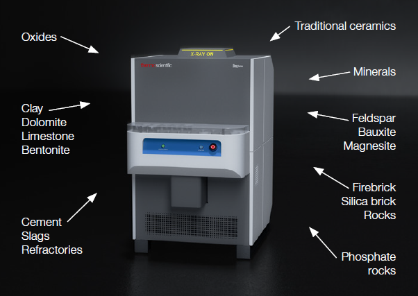
Figure 1. Many different materials can be analyzed with an ARL X900 Spectrometer calibrated with our General Oxide calibration. Image Credit: Thermo Fisher Scientific
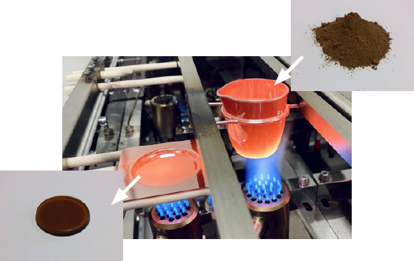
Figure 2. Transformation of the powder material into a glassy sample by fusion at high temperature. Image Credit: Thermo Fisher Scientific
Calibration Ranges, Detection Limits, and Analytical Precision
The oxide types and concentration ranges that can be addressed are displayed in Table 1. For each element, a working curve is established using the multivariable regression incorporated in the Thermo Scientific™ OXSAS™ Analysis Software package. Theoretical alpha factors are applied for all matrix corrections.
Loss on ignition values, which reach up to 47 %, can be used for correction purposes in the multivariable regression. A measure of analysis accuracy, the standard error of estimate (SEE) represents the average error between the certified concentrations of the standard samples and the calibration curve for a given oxide.
The limits of detection (LOD) obtained from low-concentration precision tests are shown in Table 2 for various oxides when the universal goniometer is used. Depending on the element and the required precision, analysis times can range from four to 40 seconds per element. When fixed-channel monochromators are used for several elements/oxides, the total counting time can be substantially reduced.
Sample Preparation
Standard samples are dried before fusion, as demonstrated in Figure 2. They are prepared as 35 mm-diameter fused beads from ignited or non-ignited powder. Ignition is performed for one hour at 1050 °C when required.
Fusion is performed using 0.7 grams of sample, 7.7 grams of flux mix (66 % Li2B4O7 - 34 % LiBO2), and 0.02 grams of LiBr (dilution 1:11) on a Katanax® Inc. electrical fusion machine or a gas fusion machine (Vulcan or FLUXANA®).
Two types of sample preparation can be used:
a. No Calcination of Samples
(→ Faster preparation for clean oxides)
Since the software estimates loss on ignition, each element must be measured for this automatic correction to function. If elements/oxides aside from the 12 measured are present, the loss on ignition should be introduced manually to enhance analysis precision.
Importantly, fusion from non-ignited samples can be fatal to the Pt-Au crucible when small metallic particles are present in the sample.
b. Fusion from Ignited Samples
(→ Improved precision and safer fusion)
Samples are ignited at 1050 °C for 1 hour to determine their loss on ignition (LOI). The ignited powder is used to prepare fused beads of 35 mm diameter. Ignited samples are easier and safer to fuse, particularly when small metallic particles are present.
Table 1. Concentration ranges of the various oxide types with the SEE achieved. Source: Thermo Fisher Scientific – Production Process & Analytics
|
|
|
0.02 g LiBr
non-wetting agent |
| Elements/ oxides |
Range (%) ignited samples |
Crystal |
Typical SEE (%)
universal gonio |
| Al2O3 |
0.2 – 90.8 |
PET |
0.16 |
| CaO |
0.02 – 98.6 |
LiF200 |
0.35 |
| Cr2O3 |
0.1 – 17.2 |
LiF200 |
0.02 |
| Fe2O3 |
0.1 – 93.8 |
LiF200 |
0.2 |
| K2O |
0.02 – 15.4 |
LiF200 |
0.03 |
| MgO |
0.05 – 95.4 |
AX06 |
0.4 |
| MnO |
0.02 – 5.5 |
LiF200 |
0.04 |
| Na2O |
0.2 – 10.06 |
AX06 |
0.07 |
| P2O5 |
0.2 – 37.7 |
PET |
0.075 |
| SO3 |
0.07 – 57 |
PET |
0.05 |
| SiO2 |
0.4 – 99.9 |
PET |
0.19 |
| TiO2 |
0.03 – 7.7 |
LiF200 |
0.03 |
Typical LODs on ARL X900 Series
Table 2. Typical limits of detection in 100 seconds obtained on various oxides using the goniometer at various power levels (fusions with 1 part sample / 11 parts flux). Source: Thermo Fisher Scientific
|
4200 W |
2500 W |
1500 W |
|
(3 sigma) (ppm) |
(3 sigma) (ppm) |
(3 sigma) (ppm) |
| CaO |
12 |
14 |
18 |
| SiO2 |
13 |
15 |
20 |
| Al2O3 |
32 |
38 |
50 |
| Fe2O3 |
12 |
14 |
18 |
| MgO |
74 |
89 |
115 |
| Na2O |
143 |
172 |
223 |
| SO3 |
17 |
20 |
26 |
| K2O |
10 |
12 |
15 |
| P2O5 |
17 |
20 |
26 |
| MnO |
8 |
9 |
12 |
| Cr2O3 |
7 |
8 |
11 |
| TiO2 |
7 |
8 |
11 |
Repeatability and Short-Term Precision in Oxide Analysis
The tables below demonstrate typical results obtained with the universal goniometer on fusion beads of various oxidic materials. Since analysis with the goniometer is sequential, elements/oxides are measured one after another.
In the first example, analyzing nine oxides requires a total of 220 seconds (Cr2O3 is not displayed as its % level fell below the detection limit).
Table 3 a. Short-term repeatability on a rock fused bead - goniometer at 20 seconds per line - 40 kV/70 mA. Source: Thermo Fisher Scientific
| Time |
20 s |
20 s |
20 s |
20 s |
20 s |
20 s |
20 s |
20 s |
20 s |
20 s |
20 s |
| Run |
CaO |
SiO2 |
Al2O3 |
MgO |
Fe2O3 |
K2O |
MnO |
Na2O |
P2O5 |
SO3 |
TiO2 |
| 1 > |
8.24 |
59.78 |
11.62 |
2.74 |
6.49 |
4.23 |
0.316 |
4.129 |
0.569 |
0.061 |
0.153 |
| 2 > |
8.28 |
59.76 |
11.64 |
2.74 |
6.49 |
4.25 |
0.318 |
4.154 |
0.573 |
0.052 |
0.151 |
| 3 > |
8.27 |
59.87 |
11.59 |
2.74 |
6.50 |
4.26 |
0.316 |
4.171 |
0.577 |
0.049 |
0.153 |
| 4 > |
8.28 |
59.71 |
11.59 |
2.73 |
6.50 |
4.25 |
0.316 |
4.164 |
0.574 |
0.052 |
0.148 |
| 5 > |
8.25 |
59.91 |
11.61 |
2.76 |
6.49 |
4.23 |
0.315 |
4.158 |
0.568 |
0.048 |
0.151 |
| 6 > |
8.28 |
59.72 |
11.70 |
2.76 |
6.49 |
4.23 |
0.316 |
4.143 |
0.572 |
0.055 |
0.152 |
| Avg |
8.26 |
59.79 |
11.63 |
2.75 |
6.49 |
4.24 |
0.316 |
4.153 |
0.572 |
0.053 |
0.151 |
| Std dev |
0.018 |
0.079 |
0.04 |
0.011 |
0.005 |
0.014 |
0.001 |
0.015 |
0.003 |
0.005 |
0.002 |
Table 3 b. Short-term repeatability on a cement-fused bead goniometer at 20 seconds per line, 40 kV/70 mA. Source: Thermo Fisher Scientific
| Time |
20 s |
20 s |
20 s |
20 s |
20 s |
20 s |
20 s |
20 s |
20 s |
20 s |
20 s |
20 s |
| Run |
CaO |
SiO2 |
Al2O3 |
MgO |
Fe2O3 |
K2O |
MnO |
Na2O |
P2O5 |
SO3 |
TiO2 |
Cr2O3 |
| 1 > |
63.65 |
20.20 |
3.701 |
2.434 |
4.850 |
0.410 |
0.190 |
0.138 |
0.075 |
2.326 |
0.153 |
0.0010 |
| 2 > |
63.61 |
20.14 |
3.651 |
2.428 |
4.866 |
0.415 |
0.185 |
0.166 |
0.072 |
2.332 |
0.156 |
0.0011 |
| 3 > |
63.65 |
20.23 |
3.715 |
2.399 |
4.846 |
0.410 |
0.188 |
0.154 |
0.073 |
2.314 |
0.154 |
0.0008 |
| 4 > |
63.62 |
20.17 |
3.651 |
2.435 |
4.862 |
0.416 |
0.186 |
0.172 |
0.073 |
2.325 |
0.158 |
0.0011 |
| 5 > |
63.71 |
20.17 |
3.707 |
2.433 |
4.856 |
0.410 |
0.189 |
0.125 |
0.072 |
2.317 |
0.152 |
0.0010 |
| 6 > |
63.62 |
20.22 |
3.665 |
2.455 |
4.866 |
0.413 |
0.189 |
0.185 |
0.075 |
2.321 |
0.156 |
0.0009 |
| Avg |
63.64 |
20.19 |
3.682 |
2.431 |
4.858 |
0.412 |
0.188 |
0.157 |
0.073 |
2.323 |
0.155 |
0.0010 |
| Std dev |
0.036 |
0.035 |
0.029 |
0.018 |
0.008 |
0.003 |
0.002 |
0.022 |
0.002 |
0.006 |
0.002 |
0.0001 |
Table 3 c. Short-term repeatability on a dolomite fused bead goniometer at 20 seconds per line, 40 kV/70 mA. Source: Thermo Fisher Scientific
| Time |
20 s |
20 s |
20 s |
20 s |
20 s |
20 s |
20 s |
20 s |
20 s |
20 s |
20 s |
| Run |
CaO |
SiO2 |
Al2O3 |
MgO |
Fe2O3 |
K2O |
MnO |
Na2O |
P2O5 |
SO3 |
TiO2 |
| 1 > |
30.86 |
0.292 |
0.065 |
21.44 |
0.448 |
0.004 |
0.073 |
0.005 |
0.0085 |
0.040 |
0.0011 |
| 2 > |
30.90 |
0.294 |
0.075 |
21.51 |
0.444 |
0.004 |
0.074 |
0.007 |
0.0081 |
0.038 |
0.0014 |
| 3 > |
30.86 |
0.291 |
0.068 |
21.54 |
0.445 |
0.004 |
0.074 |
0.009 |
0.0084 |
0.039 |
0.0010 |
| 4 > |
30.88 |
0.294 |
0.066 |
21.49 |
0.446 |
0.004 |
0.074 |
0.001 |
0.0096 |
0.044 |
0.0015 |
| 5 > |
30.90 |
0.300 |
0.069 |
21.56 |
0.446 |
0.004 |
0.075 |
0.012 |
0.0091 |
0.046 |
0.0012 |
| 6 > |
30.88 |
0.293 |
0.067 |
21.53 |
0.447 |
0.004 |
0.073 |
0.001 |
0.0085 |
0.035 |
0.0021 |
| Avg |
30.88 |
0.294 |
0.068 |
21.51 |
0.446 |
0.004 |
0.074 |
0.006 |
0.0087 |
0.040 |
0.0011 |
| Std dev |
0.019 |
0.003 |
0.003 |
0.043 |
0.001 |
0.0005 |
0.0010 |
0.005 |
0.0054 |
0.004 |
0.0004 |
Note that due to the dilution, Na2O is at the Limit of detection, hence the poor standard deviation.
Analysis with fixed monochromator channels allows quicker analysis and equal or better accuracy.
Factory Pre-Calibration and Instrument Configuration Options
The ARL X900 WDXRF Spectrometer can be pre-calibrated at the factory before shipment. Thermo Scientific uses a series of certified standard samples prepared on a Katanax electrical fusion machine or a gas fusion machine (Vulcan VAA2 or FLUXANA VITRIOX® Gas, based on customer preference).
Although the standard samples are not delivered with this pre-calibration, a set of six stable, polished setting-up samples is provided for long-term calibration curve maintenance.
Alternatively, a kit of 24 internationally certified standards of oxide materials can be ordered to support on-site instrument calibration using the client’s own sample preparation equipment.
Conclusion: WDXRF with Fusion Bead Preparation for Total Oxide Analysis
These results demonstrate that a wide range of minerals, raw materials, and oxidic products can be analyzed with excellent precision and accuracy by combining wavelength-dispersive X-ray fluorescence with a sample preparation method, such as fusion beads.
Thanks to intelligent power management, the ARL X900 Spectrometer can operate at 1500 W and 2500 W without requiring external water cooling, eliminating the need for tap water or water coolers. At higher power levels (4.2 kW), intelligent power management reduces energy consumption and minimizes stress on the X-ray tube.
The ARL X900 Spectrometers can be configured with a single sequential goniometer or with additional fixed channels to accelerate response time. These devices operate without the need for compressed air and use a minimal flow of P10 detector gas.
Finally, the OXSAS Analytical Software running on the latest Windows® environment provides extensive analytical functions and ease of use.
By combining wavelength-dispersive X-ray fluorescence with controlled fusion bead sample preparation, the ARL X900 Series WDXRF spectrometer provides a robust analytical approach for total oxide analysis across a wide range of minerals and oxidic materials. The integration of multivariable regression, matrix correction models, and flexible instrument configurations supports high analytical precision and long-term method stability in industrial and research environments.
Acknowledgements
Produced from materials originally authored by Didier Bonvin, Thermo Fisher Scientific, Ecublens, Switzerland.

This information has been sourced, reviewed, and adapted from materials provided by Thermo Fisher Scientific – Production Process & Analytics.
For more information on this source, please visit Thermo Fisher Scientific – Production Process & Analytics.